SPACE
The final frontier
The following article explores some key concepts in creating VR-ready, high quality technical art for a space exploration game.
The goal was to create a set of awe-inspiring stereoscopic visuals that would allow players closely experience celestial phenomena that would usually only be seen in science.
Space is full of interesting entities that would be challenging to create using traditional polygon-based 3D techniques, largely due to their fluid or gaseous makeup.
Raymarching is a rendering technique that involves the use of 3D vector math to project rays from a virtual camera, through a virtual space (generally one or more rays per pixel). As the rays move, we can use mathematical principles such as projection, noise functions, and color accumulation to compute an appropriate color for a given pixel.
This technique allows for atmospheric effects, custom light diffusion, procedural animation, nonlinear ray projection, and more.
Trace
Until you're out of space
To start raymarching inside a game engine, such as Unity, we first need to set up a system for per-pixel ray traversal. For spatially bounded objects, such as stars (rather than unbounded, such as infinite volumes), an inverted, low-poly sphere serves as an appropriate surface for a pixel shader.
Using a standard Unity GameObject provides access to the built-in unity_WorldToObject matrix in our shader, so we can perform our operations in Object space. This simplifies transformations and makes it easier to position, rotate, or scale the effect using typical Unity tools.
We use front-face culling on the sphere to ensure that our pixel shader runs even when our camera is inside the spherical volume. By manually tracing spherical depth inside our pixel shader, we can construct a raymarching system which is decoupled from its base geometry, giving a perfectly spherical result with no visible polygons.
struct RaymarchingInfo
{
    float3 ro; // Ray Origin
    float3 rd; // Ray Direction
    float3 p; // Position
    float minDist; // RO -> Closest front face
    float maxDist; // RO -> Furthest back face
};
RaymarchingInfo prepareSphereRaycasting(float3 worldPos)
{
    // Transpose the WorldToObject matrix to invert the rotation component
    float4x4 worldToSphericalBody = transpose(unity_WorldToObject);

    // Start at the camera, ray forward
    float3 ro = mul(float4(_WorldSpaceCameraPos, 1.0), worldToSphericalBody);
    float3 rd = normalize(mul(worldPos - _WorldSpaceCameraPos, worldToSphericalBody));

    // Find the intersection with the mesh sphere
    float2 intersection = RaySphereIntersect(ro, rd, float3(0, 0, 0), 0.5);
    float minDist = min(intersection.x, intersection.y);
    float maxDist = max(intersection.x, intersection.y);

    // Find the point from RO along RD the intersects our geometry.
    float3 p = ro + (rd * max(0, minDist));

    RaymarchingInfo info;
    info.ro = ro;
    info.rd = rd;
    info.p = p;
    info.minDist = minDist;
    info.maxDist = maxDist;

    return info;
}
Raymarching Preparation
Shader Function
Our prepareSphereRaycasting function takes the pixel position, in world space, and computes the approach object space variables for use in raymarching.
RO - The Ray Origin. This is the camera position
RD - The Ray Direction. This is the normalized vector from the camera to the pixel being rendered.
P - The Position. This is the first position to sample our field against. It's shown here as the leftmost white dot where the ray intersects with the GEOMETRY. When the camera is inside our geometry, this will be equal to RO
MinDist / MaxDist - Scalar distances to the geometry sphere intersections.
Stepping
In the above example, we use small blueish dots to indicate where a constant sample count of 5 would sample. Note that the step distance increases in rays that don't reach the core. This is an intentional tradeoff to help keep pixel cost constant. You could use constant step distances, or a hybrid solution where you have a higher fixed step count on atmospheric traces.
In the case of a black hole, the ray direction must be continuously adjusted, bending inward toward the singularity.
We use a simple ray projection to check the minimum distance to the singularity along our initial (straight) ray direction; That can be used as a heuristic to adjust the number of steps we expect to march.
We use is substepping; stepping more,shorter distances when we expect higher warping, but without additional field sampling; this helps keep the pixel cost down where more stepping is required, but more sampling isn't.
Note how rays that graze the event horizon are bent sufficiently to reach the accretion disc, but not enough to actually fall past the event horizon. It's these rays that give us the interesting warped disc that appears like a ring around the hole.
Rays that are warped, but don't hit the accretion disc (shown here in grey) would ideally sample their colour from the skydome using their (now warped) ray direction. This would give a refractive effect around the fringes of the black hole.
For the Nebula effect, we use a slightly different approach. Rather than using a fixed ray length (inferred by a fixed step count over a known distance), the Nebula uses a variable ray length with a accumulated colour function.
Here, we sample a 3D noise field, and use the returned density value to modulate the ray length for the next step - Areas of low density are interpreted as longer steps, and high density areas lead to shorter steps. Since shorter steps mean more steps to cover the same distance, this results in brighter regions.
It's important to keep ray length within sensible ranges, as overly-short rays will mean we run out of iterations before reaching the far side of our geometry.
One interesting side effect of this approach is the ability to defocus areas (such as at the outer edge of our intended region) but artificially increasing the ray length.
We need to be careful that our highest ray length doesn't accidentally "step over" regions of interest, so we clamp it. This means we have a theoretical minimum number of steps that occur across our domain, which leads to a "haze" of samples accumulated even where density is low. We can compensate for this after the trace to bring our background back down.
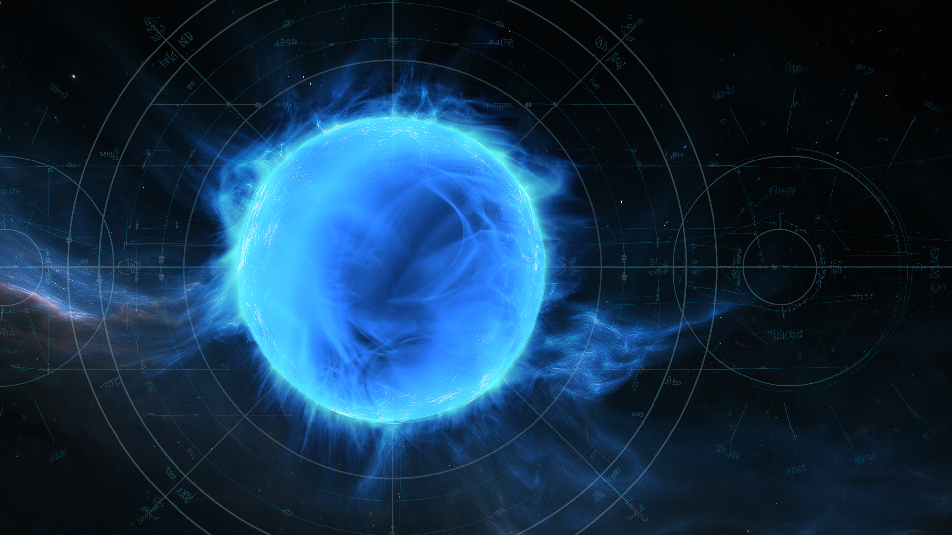
For the Neutron Star effect, we use a fixed step count, and sample against a density field, which is used to drive alpha contribution. Colour values are interpolated based on distance from CORE to P.
Shown here is the function used to calculate the density of atmosphere at a given point. After this density calculation, further calculations are applied to lower density as we move away from the core surface.
Since most interesting noise has no heuristic for ray length, we need to prioritise optimisation of our core map(float3 p) function, to allow a high step count.
In this case, we're using an FBM of a swizzled complex square root function, where each iteration of the FBM has its domain rotated by a compounding rotation matrix. By adjusting the rotation matrix per iteration, and over time, we can layer up different movements (and resolution/gain) per step, giving a mix of localised frequencies. This is especially important since the complex square root function uses abs to "fold" the domain into the positive quadrant, giving some symmetrical results, which we can diminish using the above technique.
The iteration count in the map function is fairly low, but consider that the function is called within an outer raymarch loop that may have more than 100 iterations, so things can get out of hand quickly.
float map(float3 p)
{
    // Store p
    float3 c = p;

    // Get a seeded-random rotation matrix, rotating on any axis over time.
    float3x3 rotationMatrix = generateMatrix();

    float strength = 1;
    float result = 0.;
    const int ITERATIONS = 7;
    for (int i = 0; i < ITERATIONS; ++i)
    {
        // Rotate the matrix by itself
        rotationMatrix = mul(rotationMatrix, rotationMatrix);

        // Rotate our domain
        float3 rotated = mul(p, rotationMatrix);

        // Modulate rotation strength
        p = lerp(p, rotated, saturate(1.0/i));

        // Store p for strength interpolation later.
        float3 oP = p;

        // Core noise function - https://www.shadertoy.com/view/MtX3Ws
        p = _NoiseGain * abs(p) / dot(p, p) - _NoiseGainOffset;
        p = lerp(oP,  csqr3(p), i == 0 ? _NoiseSquareBlend/2 : _NoiseSquareBlend);
        p = p.zxy;
        result += exp(-1 * _NoiseExponent * abs(dot(p, c))) * strength;

        // Reduce strength per iteration
        strength *= 0.95;
    }

    return result / 2.0;
}